By Matthew Barstead, Ph.D. | January 19, 2019
Spurred on by Alex Shackman, I have been working to figure out a good way to visualize different sources of variation in momentary mood. The most common way of visually depicting variance decompositions from the sort of multilevel models we used to analyze our data is a stacked bar plot. So that seemed like a good place to start.
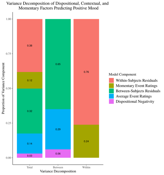
Figure 1. Stacked Barplot of Model Variance Decomposition
Now, choosing a color scheme that screams “HI I’M A COLOR!!” is one reasonable critique of this image. But, my more pressing issue is that this image, while accurately representing our model results asks a lot of the reader. You have to move back and forth between the legend and the graph to effectively map the different sources of explained variance onto their segments in the bar plot. Additioanlly, the denominator for the variance calculations shifts as you move across the x axis, and it may not be obvious to readers with passing familiarity of these models how the stacked bar plots in the right 2 columns merge together to form the stacked bar plot in the “Total” variance column. Relatedly, there is no place in this image to easily represent the total variance accounted for by between-subjects factors and within-subjects factors separately.
Unsatisfied with this graph, I played around with a number of different visualization approaches. Here is another attempt in which I tried to use the posterior distribution from our mood models, separate color schemes for between- and within-subjects sources of variation, and pie charts to provide a different visual breakdown of the variance terms. Within the violin plot on the left, I think I was going for something like the fundraising thermometer image churches place on roadsides to indicate how close they are to getting that new roof or expanding their parking lots.
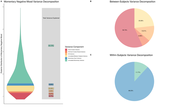
Figure 2. Pie chart version of variance decomposition
I liked the idea of including the posterior distibution from the models in this way so the reader could see that our model results mirrored the obtained data and our general expectation that negative mood is positively skewed in a relatively healthy population like the one we sampled. However, I did not like the execution of this vision, which yielded a busy plot that still requires a lot of work on the part of the reader to decipher the meaning of its components.
I knew there had to be a more elegant way to visually relate our findings to a reader. Data visualization after all should easliy summarize findings in a straightforward, transparent, and easy to digest way. These images are perhaps transparent in their representation of model results, but the are not straightforward and they are not easy to digest.
Enter the Sankey Plot
So I did what all good researchers and data scientists do when they hit a wall, I searched the Internet for solutions. Here are just a couple of links I found helpful in my digital quest: Top 50 ggplot2 Visualizations and The R Graph Gallery. It was on this latter site that I came across the Sankey Diagram. I immediately saw the potential to separate out between- and within-subjects variance, but also show how they combine to form the total variability in our dependent measure.
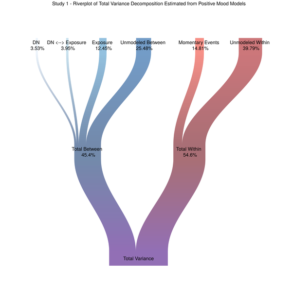
Figure 3. The riverplot we deserve
This image ticks all of my data visualization boxes, and, in my opinion, does a better job of representing what it is multilevel models do in terms of partitioning variance from multiple levels of the data. The remainder of this post is dedicated to how I got to this final plot. I will be including code from our models and I need to strongly recommend data scientists and researchers read (Rights and Sterba 2018). For related discussions and adapting the approach for non-Gaussian distributed outcomes see (Jaeger et al. 2017; Nakagawa and Schielzeth 2016). The r2mlm function Rights and Sterba created as part of their variance decomposition framework was instrumental in terms of my ability to extract the relevant variance components from our different models.
(As an aside, Jason Rights was quick to respond to an email request of mine and re-uploaded his function after I had informed him that the original formatting on his site made it difficult to easily copy and paste into R. Thanks Jason!)
The remainder of this post is going to be a walkthrough, with code snippets, of how I used the r2mlm function to extract variance components from our models and eventually create a plot the ticked all my nerdy data visualization boxes. This work is all part of a manuscript that will be sumbitted soon for publication, but I want to be upfront and say that the final products of that manuscript may not reflect exactly what you read here in this blog post.
I am going to provide a little background on our models and hypotheses, but it will not be exhaustive. I hope it is enough context to effectively understand how one might adapt this approach to their own multilevel data problems.
Methods and Background
There are numerous good resources out there that explain the basics of multilevel modeling (Gelman et al. 2013; Gelman and Hill 2007; Raudenbush and Bryk 2002), and the goal of this post is not to recapitulate what is often a semester-long graduate course in the use of these models. Briefly, these models separate out sources of variability in nested data structures. The nesting can be individuals within groups (i.e., students within classrooms) or observations within individuals (i.e., repeated sampling of the same subjects).
Dr. Shackman’s data fall into this latter category. He and his collaborators designed a study in which college students responded to 10 survey prompts throughout the day, for an entire week (yielding up to 70 observations per participant). Along with basic questions about recent activities and social surroundings, participants provided information about how they felt at the moment they were responding to the survey (i.e., measures of negative and positive mood). They also rated how pleasant the “Best” event was that happened to them since the last prompt and how distressing the “Worst” event was that had occurred since their last survey.
A key construct in Dr. Shackman’s work is dispositional negativity - which is a risk factor for a host of undesirable and interconnected outcomes (Shackman, Stockbridge, et al. 2016, 2018; Shackman, Tromp, et al. 2016; Shackman, Weinstein, et al. 2018). Where I come in is attempting to use his data to illustrate how it is dispositional negativity contributes to momentary mood and reactions to recent negative and positive events. I took the data from his 127 participants and, using Bolger and Schilling (1991) as a guide, set about the task of testing the different processes that link dispositional negativity to momentary affect.
One component of this research was separating out the unique variance explained by dispositional negativity from its shared variance with overall exposure to less positive and more negative daily events. To understand how this worked from a modeling standpoint, see the equations and walkthrough below. For simplicity’s sake I will be focusing solely on the positive mood model.
Decomposing Variance from Single Model
The key innovation provided by Rights and Sterba (2018) with their integrated variance decomposition framework is the ability to extract \(R^2\) values from multiple levels of a single multilevel model. Prior to the publication of this new technique, parsing sources of explained variance in a multilevel model was a non-trivial challenge that required multiple separate models and could occaisionally yield unsatisfactory results, including negative \(R^2\) values (Gelman & Hill, 2007; Rights & Sterba, 2018).
We adapted the Rights and Sterba approach to our data and hypotheses and utilized their r2MLM function to partition between- and within-subjects sources of variation in our momentary mood variables. Because we hoped to isolate the total, unique, and shared (with exposure) variation in momentary mood accounted for by our primary predictor dispositional negativity, we did have to run several models in which we varied which level-2 predictors. The level-1 equation for each of these models remained constant and level-1 predictors were group-mean centered as a means of maintaining the separation of between- and within-subjects sources of variability in the model.
Level 1 Equation:
\[ \begin{aligned} Y_{ti} = \pi_{0i} + \pi_{1i}(NegEvent_{ti} - \bar{NegEvent_{.i}}) + \pi_{2i}(PosEvent_{ti} - \bar{PosEvent_{.i}}) + e_{ti} \end{aligned} \]
Our models diverged in their inclusion of predictors at the second level of the model. Model 1, which we used to examine the overall effect of dispositional negativity on momentary mood, included standardized dispositional negativity scores as the sole level-2 predictor.
Model 1 Level-2 Equations:
\[
\begin{aligned}
\pi_{0i} = \beta_{00} + \beta_{01}(DN_i) + r_{0i} \\
\pi_{1i} = \beta_{10} + r_{1i} \\
\pi_{2i} = \beta_{20} + r_{2i}
\end{aligned}
\]
In R the model was estimated using brms, a wraparound package developed for Bayesian regression models that draws on Stan a general purpose Bayesian modeling program (Bürkner 2017).
Pos_lv2_DN<-brms::brm_multiple(T.PosAff~1+c.Worst+c.Best+
                                 c.DN+
                                 (1+c.Worst+c.Best|ID),
                               data = dat.study1.list,
                               family = 'normal',
                               prior = c(set_prior('student_t(3,0,1)', class='sd'),
                                         set_prior('normal(3.104,2)', class='Intercept'),
                                         set_prior('normal(0,5)', class='b'),
                                         set_prior('lkj(2)', class='cor')),
                               warmup = 2000,
                               iter = 3000,
                               chains = 3,
                               control = list(adapt_delta=.99,
                                              max_treedepth=15),
                               save_model = paste0(stan.code, '/S1_lv2a.stan'))
The brm_multiple function integrates the results from the 20 imputed data sets we created to address missing survey responses in the data. If you do not have missing data, or you want to use a frequentist approach you will have to modify this walkthrough a little, and it will be more difficult to generate 95% Highest density intervals for variance estimates (which I can do by repeatedly drawing parameter estimates from the posterior distributions and re-calculating my \(R^2\) terms).
To separately evaluate the overall effect of exposure (i.e., the tendency to report more negative and/or more positive events), Model 2 included individual averages of reported negative and positive events. These are sometimes referred to in the literature as contextual effects.
Model 2 Level-2 Equations:
\[ \begin{aligned} \pi_{0i} = \beta_{00} + \beta_{01}(\bar{NegEvent_{.i}}) + \beta_{02}(\bar{PosEvent_{.i}}) + r_{0i} \\ \pi_{1i} = \beta_{10} + r_{1i} \\ \pi_{2i} = \beta_{20} + r_{2i} \end{aligned} \]
In R…
Pos_lv2_Evnt<-brms::brm_multiple(T.PosAff~1+c.Worst+c.Best+
                                   mean.Worst+mean.Best+
                                   (1+c.Worst+c.Best|ID),
                                 data = dat.study1.list,
                                 family = 'normal',
                                 prior = c(set_prior('student_t(3,0,1)', class='sd'),
                                           set_prior('normal(3.104,2)', class='Intercept'),
                                           set_prior('normal(0,5)', class='b'),
                                           set_prior('lkj(2)', class='cor')),
                                 warmup = 2000,
                                 iter = 3000,
                                 chains = 3,
                                 control = list(adapt_delta=.99,
                                                max_treedepth=15),
                                 save_model = paste0(stan.code, '/S1_lv2b.stan'))
Finally, we included all three individual-level predictors in Model 3. Doing so allowed us to separately calculate the unique and shared variability in momentary mood attributable to dispositional negativity and overall exposure to positive and negative daily events:
Model 3 Level-2 Equations:
\[ \begin{aligned} \pi_{0i} = \beta_{00} + \beta_{01}(DN_i) + \beta_{02}(\bar{NegEvent_{.i}}) + \beta_{03}(\bar{PosEvent_{.i}}) + r_{0i} \\ \pi_{1i} = \beta_{10} + r_{1i} \\ \pi_{2i} = \beta_{20} + r_{2i} \end{aligned} \]
In R…
Pos_lv2_All<-brms::brm_multiple(T.PosAff~1+c.Worst+c.Best+
                                  mean.Worst+mean.Best+c.DN+
                                  (1+c.Worst+c.Best|ID),
                                data = dat.study1.list,
                                family = 'normal',
                                prior = c(set_prior('student_t(3,0,1)', class='sd'),
                                          set_prior('normal(3.104,2)', class='Intercept'),
                                          set_prior('normal(0,5)', class='b'),
                                          set_prior('lkj(2)', class='cor')),
                                warmup = 2000,
                                iter = 3000,
                                chains = 3,
                                control = list(adapt_delta=.99,
                                               max_treedepth=15),
                                save_model = paste0(stan.code, '/S1_lv2c.stan'))
Differences in between-subjects and total variance in momentary mood explained by each of these models formed the basis of our overall variance attributable to DN (\(R_{M1}^2\)), unique variance associated with DN (\(R_{M3}^2 - R_{M1}^2\)), and variance shared between DN and exposure (\(R_{M3}^2 - [R_{M3}^2 - R_{M1}^2]\)), where \(R^2s\) could represent total variability or be isolated solely to between-subjects variability in momentary mood and \(M1\), \(M2\), and \(M3\) represent terms extracted from Models 1, 2, and 3 respectively. To complete our understanding of sources of between subjects variability in our models, we also estimated the variance explained by an individual’s average exposure to positive and negative events (\(R_{M3}^2 - R_{M2}^2\)).
As noted above a strength of this Bayesian modeling approach is that we were able to draw parameter estimates from the posterior distributions implied by our models and calculate 95% highest density intervals for our various \(R^2\) terms of interest across the imputed data sets.
Extracting Relevant Variance Terms using r2mlm
My approach to using this function is a little bit complicated because of the multiple imputations and the need to isolate specific variance terms from each model. If you do not have missing data (email me immediately and tell me your secrets), not everything I am about to do is necessary. Also if you do not have a posterior distribution to draw from, you won’t need to get a vector of \(R^2s\). Just running the r2mlm function once for each model will be sufficient.
First, I need to collect information to pass along to the r2mlm function, including the columns in my data that correspond to my variables in the model.
#Attempting Variance Partionining for DN alone
within_cov<-c(21,23)                    #Columns with group-mean centered predictors
between_cov<-c(6)                       #Columns with between-subject predictors
random_cov<-c(21,23)                    #Level 1 predictors with random slopes
Next I extract the posterior distributions for my parameters as follows.
#Getting distributions of fixed effects
Intercept<-posterior_samples(Pos_lv2_DN, pars = 'b_Intercept')
DN<-posterior_samples(Pos_lv2_DN, pars = 'b_c.DN')
Worst<-posterior_samples(Pos_lv2_DN, pars = 'b_c.Worst')
Best<-posterior_samples(Pos_lv2_DN, pars = 'b_c.Best')

#Getting between-subjects variance terms for random effects
Int_var<-posterior_samples(Pos_lv2_DN, pars = 'sd_ID__Intercept')^2
Worst_var<-posterior_samples(Pos_lv2_DN, pars = 'sd_ID__c.Worst')^2
Best_var<-posterior_samples(Pos_lv2_DN, pars = 'sd_ID__c.Best')^2
I am going to need a covariance matrix for my random effects in each model. Luckily this is relatively straightforward as long as you can remember that \(Cov(x,y) = r_{xy} sd_x sd_y\).
#Getting covariances of random effects (i.e., tau matrix)
cov_Int_Worst<-posterior_samples(Pos_lv2_DN, pars = 'sd_ID__Intercept')*
  posterior_samples(Pos_lv2_DN, pars = 'sd_ID__c.Worst')*
  posterior_samples(Pos_lv2_DN, pars = 'cor_ID__Intercept__c.Worst')

cov_Int_Best<-posterior_samples(Pos_lv2_DN, pars = 'sd_ID__Intercept')*
  posterior_samples(Pos_lv2_DN, pars = 'sd_ID__c.Best')*
  posterior_samples(Pos_lv2_DN, pars = 'cor_ID__Intercept__c.Best')

cov_Worst_Best<-posterior_samples(Pos_lv2_DN, pars = 'sd_ID__c.Worst')*
  posterior_samples(Pos_lv2_DN, pars = 'sd_ID__c.Best')*
  posterior_samples(Pos_lv2_DN, pars = 'cor_ID__c.Worst__c.Best')
Last but not least, I need the level-1 residuals (i.e., \(\sigma_e^2\))
#Getting level 1 error variance
sigma<-posterior_samples(Pos_lv2_DN, pars = 'sigma')
Having the main components it is time for some cleanup so that I can begin extracting variance terms from my model.
post_samples<-data.frame(Intercept,
                         DN,
                         Worst,
                         Best,
                         Int_var,
                         Worst_var,
                         Best_var,
                         cov_Int_Worst,
                         cov_Int_Best,
                         cov_Worst_Best,
                         sigma)

colnames(post_samples)<-c('Intercept',
                          'DN',
                          'Worst',
                          'Best',
                          'Int_var',
                          'Worst_var',
                          'Best_var',
                          'cov_Int_Worst',
                          'cov_Int_Best',
                          'cov_Worst_Best',
                          'sigma')
I mentioned before that I am going to be taking a Bayesian approach here, which means sampling repeatedly from my posterior distributions. This approach is complicated slightly by the fact that my posterior distributions are unique to each of the 20 datasets I imputed. This means I need to be deliberate about how I sample from the posterior and which of the 20 data sets I apply the sampled parameter estimates to when running the r2mlm function. The code below makes this happen and extracts the variance terms of interest for my final graphic.
#Aggregate across imputed datasets
#Currently going to take 1000 draws from posterior distributions
#Will then apply across all 20 data sets

P_DN_alone<-list(between_var=vector(),
               within_var=vector(),
               between_All_tot=vector(),
               between_All_btw=vector(),
               between_res_btw=vector(),
               within_fix_wthn=vector(),
               within_fix_tot=vector(),
               within_slope_var_wthn=vector(),
               within_res_wthn=vector(),
               within_unmod_tot=vector())

#Will be used to line up posterior distributions
#Because  posterior parameter estimates are unique to each imputed data set
#Probably ways to make this more programmatically fluid...
sampling_list<-list(imp1 = 1:3000,
                    imp2 = 1:3000 + 3000,
                    imp3 = 1:3000 + 6000,
                    imp4 = 1:3000 + 9000,
                    imp5 = 1:3000 + 12000,
                    imp6 = 1:3000 + 15000,
                    imp7 = 1:3000 + 18000,
                    imp8 = 1:3000 + 21000,
                    imp9 = 1:3000 + 24000,
                    imp10 = 1:3000 + 27000,
                    imp11 = 1:3000 + 30000,
                    imp12 = 1:3000 + 33000,
                    imp13 = 1:3000 + 36000,
                    imp14 = 1:3000 + 39000,
                    imp15 = 1:3000 + 42000,
                    imp16 = 1:3000 + 45000,
                    imp17 = 1:3000 + 48000,
                    imp18 = 1:3000 + 51000,
                    imp19 = 1:3000 + 54000,
                    imp20 = 1:3000 + 57000)

for(i in 1:length(dat.study1.list)){
  print(paste('Starting w/ imputed set', i, 'out of', M))
  D<-sample(sampling_list[[i]], size = 1000, replace = FALSE)
  for(d in 1:length(D)){
    #browser()
    Gamma_w<-as.vector(
      as.matrix(
        post_samples[D[d], c('Worst', 'Best')]))       #Make sure the effects line up - in order of within_cov
    Gamma_b<-as.vector(
      as.matrix(
        post_samples[D[d], c('Intercept', 'DN')]))    #level fixed intercept and any level 2 fixed effects
    tau<-c(post_samples[D[d], c('Int_var', 'cov_Int_Worst', 'cov_Int_Best')],
           post_samples[D[d], c('cov_Int_Worst', 'Worst_var', 'cov_Worst_Best')],
           post_samples[D[d], c('cov_Int_Best', 'cov_Worst_Best', 'Best_var')])

    tau<-matrix(unlist(tau),
                byrow=TRUE,
                ncol=3)

    #Matrix rows/columns ordered starting with tau.00 (intercept variance)
    #then add columns/rows for random effects of slopes in order of within_cov

    Sigma2<-post_samples[D[d], 'sigma']

    r2mlm_DN<-r2MLM(data=dat.study1.list[[i]],
                    within_covs = within_cov,
                    between_covs = between_cov,
                    random_covs = random_cov,
                    gamma_w = Gamma_w,
                    gamma_b = Gamma_b,
                    Tau = tau,
                    sigma2 = Sigma2,
                    has_intercept = TRUE,
                    clustermeancentered = TRUE)

    #Extracting relevant values across imputed datasets
    P_DN_alone$between_var<-c(P_DN_alone$between_var, as.numeric(r2mlm_DN$Decompositions['fixed, between', 'total'])+
                              as.numeric(r2mlm_DN$Decompositions['mean variation', 'total']))
    P_DN_alone$within_var<-c(P_DN_alone$within_var, as.numeric(r2mlm_DN$Decompositions['sigma2', 'total'])+
                             as.numeric(r2mlm_DN$Decompositions['slope variation', 'total'])+
                             as.numeric(r2mlm_DN$Decompositions['fixed, within', 'total']))
    P_DN_alone$between_All_tot<-c(P_DN_alone$between_All_tot, as.numeric(r2mlm_DN$R2s['f2', 'total']))
    P_DN_alone$between_All_btw<-c(P_DN_alone$between_All_btw, as.numeric(r2mlm_DN$R2s['f2', 'between']))
    P_DN_alone$between_res_btw<-c(P_DN_alone$between_res_btw, as.numeric(r2mlm_DN$R2s['m', 'between']))
    P_DN_alone$within_fix_wthn<-c(P_DN_alone$within_fix_wthn, as.numeric(r2mlm_DN$Decompositions['fixed, within', 'within']))
    P_DN_alone$within_fix_tot<-c(P_DN_alone$within_fix_wthn, as.numeric(r2mlm_DN$Decompositions['fixed, within', 'total']))
    P_DN_alone$within_slope_var_wthn<-c(P_DN_alone$within_slope_var, as.numeric(r2mlm_DN$Decompositions['slope variation', 'within']))
    P_DN_alone$within_res_wthn<-c(P_DN_alone$within_res_wthn, as.numeric(r2mlm_DN$Decompositions['sigma2', 'within']))
    P_DN_alone$within_unmod_tot<-c(P_DN_alone$within_unmod_wthn, as.numeric(r2mlm_DN$Decompositions['sigma2', 'total'])+
                                   as.numeric(r2mlm_DN$Decompositions['slope variation', 'total']))

    print(paste("Sampling", d, "out of", length(D), '- Dataset:', i))
  }
  print(paste("*** Finshed imputed data set", i, 'out of', M, "***"))
}
I then repeat this approach with the average event ratings as the sole predictors of the intercept.
#Event only model (these are context effects on intercept)
within_cov<-c(21,23)                    #Columns with group-mean centered predictors
between_cov<-c(22, 24)                  #Columns with between-subject predictors
random_cov<-c(21,23)                    #Level 1 predictors with random slopes

#Getting distributions of fixed effects
Intercept<-posterior_samples(Pos_lv2_Evnt, pars = 'b_Intercept')
M.Worst<-posterior_samples(Pos_lv2_Evnt, pars = 'b_mean.Worst')
M.Best<-posterior_samples(Pos_lv2_Evnt, pars = 'b_mean.Best')
Worst<-posterior_samples(Pos_lv2_Evnt, pars = 'b_c.Worst')
Best<-posterior_samples(Pos_lv2_Evnt, pars = 'b_c.Best')

#Getting between-subjects variance terms for random effects
Int_var<-posterior_samples(Pos_lv2_Evnt, pars = 'sd_ID__Intercept')^2
Worst_var<-posterior_samples(Pos_lv2_Evnt, pars = 'sd_ID__c.Worst')^2
Best_var<-posterior_samples(Pos_lv2_Evnt, pars = 'sd_ID__c.Best')^2

#Getting covariances of random effects (i.e., tau matrix)
cov_Int_Worst<-posterior_samples(Pos_lv2_Evnt, pars = 'sd_ID__Intercept')*
  posterior_samples(Pos_lv2_Evnt, pars = 'sd_ID__c.Worst')*
  posterior_samples(Pos_lv2_Evnt, pars = 'cor_ID__Intercept__c.Worst')

cov_Int_Best<-posterior_samples(Pos_lv2_Evnt, pars = 'sd_ID__Intercept')*
  posterior_samples(Pos_lv2_Evnt, pars = 'sd_ID__c.Best')*
  posterior_samples(Pos_lv2_Evnt, pars = 'cor_ID__Intercept__c.Best')

cov_Worst_Best<-posterior_samples(Pos_lv2_Evnt, pars = 'sd_ID__c.Worst')*
  posterior_samples(Pos_lv2_Evnt, pars = 'sd_ID__c.Best')*
  posterior_samples(Pos_lv2_Evnt, pars = 'cor_ID__c.Worst__c.Best')

#Getting level 1 error variance
sigma<-posterior_samples(Pos_lv2_Evnt, pars = 'sigma')
post_samples<-data.frame(Intercept,
                         M.Worst,
                         M.Best,
                         Worst,
                         Best,
                         Int_var,
                         Worst_var,
                         Best_var,
                         cov_Int_Worst,
                         cov_Int_Best,
                         cov_Worst_Best,
                         sigma)

colnames(post_samples)<-c('Intercept',
                          'M.Worst',
                          'M.Best',
                          'Worst',
                          'Best',
                          'Int_var',
                          'Worst_var',
                          'Best_var',
                          'cov_Int_Worst',
                          'cov_Int_Best',
                          'cov_Worst_Best',
                          'sigma')
#Aggregate across imputed datasets
#Currently going to take 1000 draws from posterior distributions
#Will then apply across all 20 data sets
P_Evnt_alone<-list(between_var=vector(),
                 within_var=vector(),
                 between_All_tot=vector(),
                 between_All_btw=vector(),
                 between_res_btw=vector(),
                 within_fix_wthn=vector(),
                 within_fix_tot=vector(),
                 within_slope_var_wthn=vector(),
                 within_res_wthn=vector(),
                 within_unmod_tot=vector())

for(i in 1:length(dat.study1.list)){
  print(paste('Starting w/ imputed set', i, 'out of', M))
  D<-sample(sampling_list[[i]], size = 1000, replace = FALSE)
  for(d in 1:length(D)){
    #browser()
    Gamma_w<-as.vector(
      as.matrix(
        post_samples[D[d], c('Worst', 'Best')]))       #Make sure the effects line up - in order of within_cov
    Gamma_b<-as.vector(
      as.matrix(
        post_samples[D[d], c('Intercept', 'M.Worst', 'M.Best')]))    #level fixed intercept and any level 2 fixed effects
    tau<-c(post_samples[D[d], c('Int_var', 'cov_Int_Worst', 'cov_Int_Best')],
           post_samples[D[d], c('cov_Int_Worst', 'Worst_var', 'cov_Worst_Best')],
           post_samples[D[d], c('cov_Int_Best', 'cov_Worst_Best', 'Best_var')])

    tau<-matrix(unlist(tau),
                byrow=TRUE,
                ncol=3)

    #Matrix rows/columns ordered starting with tau.00 (intercept variance)
    #then add columns/rows for random effects of slopes in order of within_cov

    Sigma2<-post_samples[D[d], 'sigma']

    r2mlm_Evnt<-r2MLM(data=dat.study1.list[[i]],
                      within_covs = within_cov,
                      between_covs = between_cov,
                      random_covs = random_cov,
                      gamma_w = Gamma_w,
                      gamma_b = Gamma_b,
                      Tau = tau,
                      sigma2 = Sigma2,
                      has_intercept = TRUE,
                      clustermeancentered = TRUE)

    #Extracting relevant values across imputed datasets
    P_Evnt_alone$between_var<-c(P_Evnt_alone$between_var, as.numeric(r2mlm_Evnt$Decompositions['fixed, between', 'total'])+
                                as.numeric(r2mlm_Evnt$Decompositions['mean variation', 'total']))
    P_Evnt_alone$within_var<-c(P_Evnt_alone$within_var, as.numeric(r2mlm_Evnt$Decompositions['sigma2', 'total'])+
                               as.numeric(r2mlm_Evnt$Decompositions['slope variation', 'total'])+
                               as.numeric(r2mlm_Evnt$Decompositions['fixed, within', 'total']))
    P_Evnt_alone$between_All_tot<-c(P_Evnt_alone$between_All_tot, as.numeric(r2mlm_Evnt$R2s['f2', 'total']))
    P_Evnt_alone$between_All_btw<-c(P_Evnt_alone$between_All_btw, as.numeric(r2mlm_Evnt$R2s['f2', 'between']))
    P_Evnt_alone$between_res_btw<-c(P_Evnt_alone$between_res_btw, as.numeric(r2mlm_Evnt$R2s['m', 'between']))
    P_Evnt_alone$within_fix_wthn<-c(P_Evnt_alone$within_fix_wthn, as.numeric(r2mlm_Evnt$Decompositions['fixed, within', 'within']))
    P_Evnt_alone$within_fix_tot<-c(P_Evnt_alone$within_fix_wthn, as.numeric(r2mlm_Evnt$Decompositions['fixed, within', 'total']))
    P_Evnt_alone$within_slope_var_wthn<-c(P_Evnt_alone$within_slope_var, as.numeric(r2mlm_Evnt$Decompositions['slope variation', 'within']))
    P_Evnt_alone$within_res_wthn<-c(P_Evnt_alone$within_res_wthn, as.numeric(r2mlm_Evnt$Decompositions['sigma2', 'within']))
    P_Evnt_alone$within_unmod_tot<-c(P_Evnt_alone$within_unmod_wthn, as.numeric(r2mlm_Evnt$Decompositions['sigma2', 'total'])+
                                     as.numeric(r2mlm_Evnt$Decompositions['slope variation', 'total']))

    print(paste("Sampling", d, "out of", length(D), '- Dataset:', i))
  }
  print(paste("*** Finshed imputed data set", i, 'out of', M, "***"))
}
And finally, I do the same with the combined model.
#Combined Level 2 Model (these are context effects on intercept)
within_cov<-c(21,23)                    #Columns with group-mean centered predictors
between_cov<-c(6, 22, 24)               #Columns with between-subject predictors
random_cov<-c(21,23)                    #Level 1 predictors with random slopes

#Getting distributions of fixed effects
Intercept<-posterior_samples(Pos_lv2_All, pars = 'b_Intercept')
DN<-posterior_samples(Pos_lv2_All, pars = 'b_c.DN')
M.Worst<-posterior_samples(Pos_lv2_All, pars = 'b_mean.Worst')
M.Best<-posterior_samples(Pos_lv2_All, pars = 'b_mean.Best')
Worst<-posterior_samples(Pos_lv2_All, pars = 'b_c.Worst')
Best<-posterior_samples(Pos_lv2_All, pars = 'b_c.Best')

#Getting between-subjects variance terms for random effects
Int_var<-posterior_samples(Pos_lv2_All, pars = 'sd_ID__Intercept')^2
Worst_var<-posterior_samples(Pos_lv2_All, pars = 'sd_ID__c.Worst')^2
Best_var<-posterior_samples(Pos_lv2_All, pars = 'sd_ID__c.Best')^2

#Getting covariances of random effects (i.e., tau matrix)
cov_Int_Worst<-posterior_samples(Pos_lv2_All, pars = 'sd_ID__Intercept')*
  posterior_samples(Pos_lv2_All, pars = 'sd_ID__c.Worst')*
  posterior_samples(Pos_lv2_All, pars = 'cor_ID__Intercept__c.Worst')

cov_Int_Best<-posterior_samples(Pos_lv2_All, pars = 'sd_ID__Intercept')*
  posterior_samples(Pos_lv2_All, pars = 'sd_ID__c.Best')*
  posterior_samples(Pos_lv2_All, pars = 'cor_ID__Intercept__c.Best')

cov_Worst_Best<-posterior_samples(Pos_lv2_All, pars = 'sd_ID__c.Worst')*
  posterior_samples(Pos_lv2_All, pars = 'sd_ID__c.Best')*
  posterior_samples(Pos_lv2_All, pars = 'cor_ID__c.Worst__c.Best')

#Getting level 1 error variance
sigma<-posterior_samples(Pos_lv2_All, pars = 'sigma')
post_samples<-data.frame(Intercept,
                         DN,
                         M.Worst,
                         M.Best,
                         Worst,
                         Best,
                         Int_var,
                         Worst_var,
                         Best_var,
                         cov_Int_Worst,
                         cov_Int_Best,
                         cov_Worst_Best,
                         sigma)

colnames(post_samples)<-c('Intercept',
                          'DN',
                          'M.Worst',
                          'M.Best',
                          'Worst',
                          'Best',
                          'Int_var',
                          'Worst_var',
                          'Best_var',
                          'cov_Int_Worst',
                          'cov_Int_Best',
                          'cov_Worst_Best',
                          'sigma')
#Aggregate across imputed datasets
#Currently going to take 1000 draws from posterior distributions
#Will then apply across all 20 data sets
P_Lv2_comb<-list(between_var=vector(),
               within_var=vector(),
               between_All_tot=vector(),
               between_All_btw=vector(),
               between_res_btw=vector(),
               within_fix_wthn=vector(),
               within_fix_tot=vector(),
               within_slope_var_wthn=vector(),
               within_res_wthn=vector(),
               within_unmod_tot=vector())

for(i in 1:length(dat.study1.list)){
  print(paste('Starting w/ imputed set', i, 'out of', M))
  D<-sample(sampling_list[[i]], size = 1000, replace = FALSE)
  for(d in 1:length(D)){
    #browser()
    Gamma_w<-as.vector(
      as.matrix(
        post_samples[D[d], c('Worst', 'Best')]))       #Make sure the effects line up - in order of within_cov
    Gamma_b<-as.vector(
      as.matrix(
        post_samples[D[d], c('Intercept', 'DN', 'M.Worst', 'M.Best')]))    #level fixed intercept and any level 2 fixed effects
    tau<-c(post_samples[D[d], c('Int_var', 'cov_Int_Worst', 'cov_Int_Best')],
           post_samples[D[d], c('cov_Int_Worst', 'Worst_var', 'cov_Worst_Best')],
           post_samples[D[d], c('cov_Int_Best', 'cov_Worst_Best', 'Best_var')])

    tau<-matrix(unlist(tau),
                byrow=TRUE,
                ncol=3)

    #Matrix rows/columns ordered starting with tau.00 (intercept variance)
    #then add columns/rows for random effects of slopes in order of within_cov

    Sigma2<-post_samples[D[d], 'sigma']

    r2mlm_All<-r2MLM(data=dat.study1.list[[i]],
                     within_covs = within_cov,
                     between_covs = between_cov,
                     random_covs = random_cov,
                     gamma_w = Gamma_w,
                     gamma_b = Gamma_b,
                     Tau = tau,
                     sigma2 = Sigma2,
                     has_intercept = TRUE,
                     clustermeancentered = TRUE)

    #Extracting relevant values across imputed datasets
    P_Lv2_comb$between_var<-c(P_Lv2_comb$between_var, as.numeric(r2mlm_All$Decompositions['fixed, between', 'total'])+
                              as.numeric(r2mlm_All$Decompositions['mean variation', 'total']))
    P_Lv2_comb$within_var<-c(P_Lv2_comb$within_var, as.numeric(r2mlm_All$Decompositions['sigma2', 'total'])+
                             as.numeric(r2mlm_All$Decompositions['slope variation', 'total'])+
                             as.numeric(r2mlm_All$Decompositions['fixed, within', 'total']))
    P_Lv2_comb$between_All_tot<-c(P_Lv2_comb$between_All_tot, as.numeric(r2mlm_All$R2s['f2', 'total']))
    P_Lv2_comb$between_All_btw<-c(P_Lv2_comb$between_All_btw, as.numeric(r2mlm_All$R2s['f2', 'between']))
    P_Lv2_comb$between_res_btw<-c(P_Lv2_comb$between_res_btw, as.numeric(r2mlm_All$R2s['m', 'between']))
    P_Lv2_comb$within_fix_wthn<-c(P_Lv2_comb$within_fix_wthn, as.numeric(r2mlm_All$Decompositions['fixed, within', 'within']))
    P_Lv2_comb$within_fix_tot<-c(P_Lv2_comb$within_fix_wthn, as.numeric(r2mlm_All$Decompositions['fixed, within', 'total']))
    P_Lv2_comb$within_slope_var_wthn<-c(P_Lv2_comb$within_slope_var, as.numeric(r2mlm_All$Decompositions['slope variation', 'within']))
    P_Lv2_comb$within_res_wthn<-c(P_Lv2_comb$within_res_wthn, as.numeric(r2mlm_All$Decompositions['sigma2', 'within']))
    P_Lv2_comb$within_unmod_tot<-c(P_Lv2_comb$within_unmod_wthn, as.numeric(r2mlm_All$Decompositions['sigma2', 'total'])+
                                   as.numeric(r2mlm_All$Decompositions['slope variation', 'total']))

    print(paste("Sampling", d, "out of", length(D), '- Dataset:', i))
  }
  print(paste("*** Finshed imputed data set", i, 'out of', M, "***"))
}
Now that I have all of the values I need for my plot, I am just a few calculations away from getting what I want. As a quick aside here, note that I can now get 95% highest density intervals for my different variance terms using different adaptations of the following code: quantile(P_DN_alone$between_All_tot, c(.025, .975)).
Using the riverplot Package
Remember this all started with a desire to get a graphic that was straightforward, transparent, and easy to digest?
Well we are almost there, but first, I need to isolate the variance explained by the dispositional negativity variable (DN) and the shared variance between DN and individual variation in the average ratings of positive and negative daily events. I also threw in the unique variance explained by average exposure to positive and negative events, above and beyond individual differences in dispositional negativity.
P_btw_DN_uni_tot<-mean(P_Lv2_comb$between_All_tot)-mean(P_Evnt_alone$between_All_tot)
P_btw_shared_tot<-mean(P_DN_alone$between_All_tot)-P_btw_DN_uni_tot
P_btw_context_uni_tot<-mean(P_Lv2_comb$between_All_tot)-mean(P_DN_alone$between_All_tot)

sum(c(P_btw_DN_uni_tot,
      P_btw_shared_tot,
      P_btw_context_uni_tot))

#The above total should equal:
mean(P_Lv2_comb$between_All_tot)

#Now getting the between subjects residual variance from final model
P_btw_res_tot<-mean(P_Lv2_comb$between_var-P_Lv2_comb$between_All_tot)
P_btw_res_tot+sum(c(P_btw_DN_uni_tot,
                    P_btw_shared_tot,
                    P_btw_context_uni_tot))
Now it is the within-subject variance I need to extract:
#Final getting the within subjects variance:
P_wthn_best_worst_tot<-mean(P_Lv2_comb$within_fix_tot)
P_wthn_res_tot<-mean(P_Lv2_comb$within_var)-P_wthn_best_worst_tot

#Should be equal to 1
sum(c(P_wthn_best_worst_tot,
      P_wthn_res_tot,
      mean(P_Lv2_comb$between_var)))
And finally the total between- and within-subjects variability estimated in the models.
P_tot_btw<-mean(P_Lv2_comb$between_var)
P_tot_wthn<-mean(P_Lv2_comb$within_var)
Using the riverplot package (Weiner 2017), I then created my Sankey diagram as follows:
River_DF<-data.frame(N1 = c('DN',
                            'DN <--> Exposure',
                            'Exposure',
                            'Unmodeled Between',
                            'Momentary Events',
                            'Unmodeled Within',
                            'Total Between',
                            'Total Within'),
                     N2 = c('Total Between',
                            'Total Between',
                            'Total Between',
                            'Total Between',
                            'Total Within',
                            'Total Within',
                            'Total Variance',
                            'Total Variance'),
                     Value = c(P_btw_DN_uni_tot,
                               P_btw_shared_tot,
                               P_btw_context_uni_tot,
                               P_btw_res_tot,
                               P_wthn_best_worst_tot,
                               P_wthn_res_tot,
                               P_tot_btw,
                               P_tot_wthn),
                     ID = 1:8)

River_DF$N1<-paste(River_DF$N1,
                   '\n',
                   paste0(round(River_DF$Value*100,
                                digits = 2), '%'
                   )
)
River_DF$N2<-c(rep(River_DF$N1[7], 4),
               rep(River_DF$N1[8], 2),
               rep('Total Variance', 2)
)

nodes<-data.frame(ID = c(River_DF$N1,
                         'Total Variance'),
                  x = c(1,1,1,1,1,1,2,2,3),
                  y = c(0,1.5,3.25,5.25,8,10.5,2.5,7.5,5))

palette = c(paste0(brewer.pal(9, "Blues"), 90)[c(2, 4, 6, 8)],
            paste0(brewer.pal(9, "Reds"), 90)[c(6, 8)],
            paste0(brewer.pal(9, "Blues"), 90)[9],
            paste0(brewer.pal(9, "Reds"), 90)[9],
            paste0(brewer.pal(9, 'Purples'), 90)[9])

styles = lapply(nodes$y, function(n) {
  list(col = palette[n], lty = 0, textcol = "black")
})

#Not sure why color is not mapping correctly with code above but it if I add this code:
for(i in 1:length(palette)){
  styles[[i]]$col<-palette[i]
}

names(styles) = nodes$ID

riv<-makeRiver(nodes = nodes,
               edges =  River_DF,
               node_styles = styles)

#Generating and saving image to my folder
png(paste0(study1.graphics, '/S1_PosMood_river.png'),
    units = 'in',
    res = 1200,
    height = 10,
    width = 10)
riverplot(riv,
          nodewidth = 3,
          plot_area = .95)
title(ylab = 'Study 1 - Riverplot of Total Variance Decomposition Estimated from Positive Mood Models')
dev.off()
And here you have it, the final result, which I rotated outside of R to be oriented vertically. The riverplot package will provide a flow that moves from left to right by default.

Figure 4 - Variance Decomposition - As Visually Straightforward as I can make it
Best of luck applying this approach to your own data. And let’s hope the reviewers of our forthcoming manuscript are sufficiently impressed with this attempt to visually present our model results.
References
Bolger, Niall, and Elizabeth A. Schilling. 1991. “Personality and the problems of everyday Life: The role of neuroticism in exposure and reactivity to daily stressors.” Journal of Personality 59 (3): 355–86. https://doi.org/10.1111/j.1467-6494.1991.tb00253.x.
Bürkner, Paul-Christian. 2017. “brms : An R Package for Bayesian Multilevel Models Using Stan.” Journal of Statistical Software 80 (1). https://doi.org/10.18637/jss.v080.i01.
Gelman, Andrew, John B. Carlin, Hal S. Stern, David B. Dunson, Aki Vehtari, and Donald B. Rubin. 2013. Bayesian data analysis. New York: CRC Press.
Gelman, Andrew, and Jennifer Hill. 2007. Data analysis using regression and multilevel/hierarchical models. New York: Cambridge University Press.
Jaeger, Byron C., Lloyd J. Edwards, Kalyan Das, and Pranab K. Sen. 2017. “An R2 statistic for fixed effects in the generalized linear mixed model.” Journal of Applied Statistics 44 (6): 1086–1105. https://doi.org/10.1080/02664763.2016.1193725.
Nakagawa, Shinichi, and Holger Schielzeth. 2016. “Coefficient of determination R2 and intra-class correlation coefficient ICC from generalized linear mixed-effects models.” Ecology and Evolution. https://doi.org/10.1101/095851.
Raudenbush, S. W., and A. S. Bryk. 2002. Hierarchical linear models: Applications and data analysis methods. 2nd ed. Thousand Oaks, CA: Sage.
Rights, Jason D., and Sonya K. Sterba. 2018. “Quantifying explained variance in multilevel models: An integrative framework for defining R-squared measures.” Psychological Methods. https://doi.org/10.1037/met0000184.
Shackman, Alexander J., Melissa D. Stockbridge, Edward P. Lemay, and Andrew S. Fox. 2018. “The psychological and neurobiological bases of dispositional negativity.” In The Nature of Emotion: Fundamental Questions2, edited by Andrew S. Fox, R. C. Lapate, Alexander J. Shackman, and R. J. Davidson, 2nd ed. New York: Oxford University Press.
Shackman, Alexander J., Melissa Stockbridge, Rachael Tillman, Claire Kaplan, Do Tromp, Andrew Fox, and Matthias Gamer. 2016. “The neurobiology of dispositional negativity and attentional biases to threat: Implications for understanding anxiety disorders in adults and youth.” Journal of Experimental Psychopathology 7 (3): 311–42. https://doi.org/10.5127/jep.054015.
Shackman, Alexander J., Do P. M. Tromp, Melissa D. Stockbridge, Claire M. Kaplan, Rachael M. Tillman, and Andrew S. Fox. 2016. “Dispositional negativity: An integrative psychological and neurobiological perspective.” Psychological Bulletin 142 (12): 1275–1314. https://doi.org/10.1037/bul0000073.
Shackman, Alexander J., Jennifer S. Weinstein, Stanton N. Hudja, Conor D. Bloomer, Matthew G. Barstead, Andrew S. Fox, and Edward P. Lemay. 2018. “Dispositional negativity in the wild: Social environment governs momentary emotional experience.” Emotion 18 (5): 707–24. https://doi.org/10.1037/emo0000339.
Weiner, January. 2017. Riverplot: Sankey or Ribbon Plots. https://CRAN.R-project.org/package=riverplot.